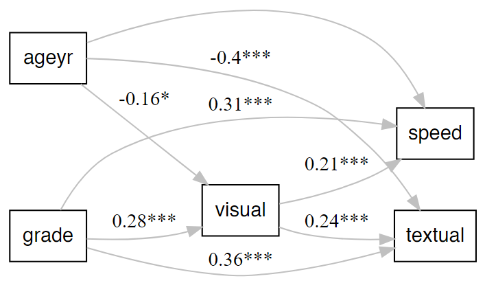
Make a quick lavaanPlot

Make a quick and decent-looking lavaanPlot.

Usage

nice_lavaanPlot(
  model,
  node_options = list(shape = "box", fontname = "Helvetica"),
  edge_options = c(color = "black"),
  coefs = TRUE,
  stand = TRUE,
  covs = FALSE,
  stars = c("regress", "latent", "covs"),
  sig = 0.05,
  graph_options = c(rankdir = "LR"),
  ...
)

Arguments

model

SEM or CFA model to plot.

node_options

Shape and font name.

edge_options

Colour of edges.

coefs

Logical, whether to plot coefficients. Defaults to TRUE.

stand

Logical, whether to use standardized coefficients. Defaults to TRUE.

covs

Logical, whether to plot covariances. Defaults to FALSE.

stars

Which links to plot significance stars for. One of c("regress", "latent", "covs").

sig

Which significance threshold to use to plot coefficients (defaults to .05). To plot all coefficients, set sig to 1.

graph_options

Read from left to right, rather than from top to bottom.

...

Arguments to be passed to function lavaanPlot::lavaanPlot.

Value

A lavaanPlot, of classes c("grViz", "htmlwidget"), representing the specified lavaan model.

Illustrations

Examples

x <- paste0("x", 1:9)
(latent <- list(
  visual = x[1:3],
  textual = x[4:6],
  speed = x[7:9]
))
#> $visual
#> [1] "x1" "x2" "x3"
#> 
#> $textual
#> [1] "x4" "x5" "x6"
#> 
#> $speed
#> [1] "x7" "x8" "x9"
#> 

HS.model <- write_lavaan(latent = latent)
cat(HS.model)
#> ##################################################
#> # [-----Latent variables (measurement model)-----]
#> 
#> visual =~ x1 + x2 + x3
#> textual =~ x4 + x5 + x6
#> speed =~ x7 + x8 + x9
#> 

library(lavaan)
fit <- cfa(HS.model, HolzingerSwineford1939)
nice_lavaanPlot(fit)