Full CFA/SEM workflow
Rémi Thériault
August 29, 2022
Source:vignettes/fullworkflow.Rmd
fullworkflow.RmdCFA example
# Load library
library(lavaan)
library(lavaanExtra)
library(tibble)
library(psych)

# Define latent variables
x <- paste0("x", 1:9)
latent <- list(
  visual = x[1:3],
  textual = x[4:6],
  speed = x[7:9]
)

# Write the model, and check it
cfa.model <- write_lavaan(latent = latent)
cat(cfa.model)
## ##################################################
## # [-----Latent variables (measurement model)-----]
##
## visual =~ x1 + x2 + x3
## textual =~ x4 + x5 + x6
## speed =~ x7 + x8 + x9
# Fit the model fit and plot with `lavaanExtra::cfa_fit_plot`
# to get the factor loadings visually (optionally as PDF)
fit.cfa <- cfa_fit_plot(cfa.model, HolzingerSwineford1939)
## lavaan 0.6-20 ended normally after 35 iterations
##
## Estimator ML
## Optimization method NLMINB
## Number of model parameters 21
##
## Number of observations 301
##
## Model Test User Model:
## Standard Scaled
## Test Statistic 85.306 87.132
## Degrees of freedom 24 24
## P-value (Chi-square) 0.000 0.000
## Scaling correction factor 0.979
## Yuan-Bentler correction (Mplus variant)
##
## Model Test Baseline Model:
##
## Test statistic 918.852 880.082
## Degrees of freedom 36 36
## P-value 0.000 0.000
## Scaling correction factor 1.044
##
## User Model versus Baseline Model:
##
## Comparative Fit Index (CFI) 0.931 0.925
## Tucker-Lewis Index (TLI) 0.896 0.888
##
## Robust Comparative Fit Index (CFI) 0.930
## Robust Tucker-Lewis Index (TLI) 0.895
##
## Loglikelihood and Information Criteria:
##
## Loglikelihood user model (H0) -3737.745 -3737.745
## Scaling correction factor 1.133
## for the MLR correction
## Loglikelihood unrestricted model (H1) -3695.092 -3695.092
## Scaling correction factor 1.051
## for the MLR correction
##
## Akaike (AIC) 7517.490 7517.490
## Bayesian (BIC) 7595.339 7595.339
## Sample-size adjusted Bayesian (SABIC) 7528.739 7528.739
##
## Root Mean Square Error of Approximation:
##
## RMSEA 0.092 0.093
## 90 Percent confidence interval - lower 0.071 0.073
## 90 Percent confidence interval - upper 0.114 0.115
## P-value H_0: RMSEA <= 0.050 0.001 0.001
## P-value H_0: RMSEA >= 0.080 0.840 0.862
##
## Robust RMSEA 0.092
## 90 Percent confidence interval - lower 0.072
## 90 Percent confidence interval - upper 0.114
## P-value H_0: Robust RMSEA <= 0.050 0.001
## P-value H_0: Robust RMSEA >= 0.080 0.849
##
## Standardized Root Mean Square Residual:
##
## SRMR 0.065 0.065
##
## Parameter Estimates:
##
## Standard errors Sandwich
## Information bread Observed
## Observed information based on Hessian
##
## Latent Variables:
## Estimate Std.Err z-value P(>|z|) Std.lv Std.all
## visual =~
## x1 1.000 0.900 0.772
## x2 0.554 0.132 4.191 0.000 0.498 0.424
## x3 0.729 0.141 5.170 0.000 0.656 0.581
## textual =~
## x4 1.000 0.990 0.852
## x5 1.113 0.066 16.946 0.000 1.102 0.855
## x6 0.926 0.061 15.089 0.000 0.917 0.838
## speed =~
## x7 1.000 0.619 0.570
## x8 1.180 0.130 9.046 0.000 0.731 0.723
## x9 1.082 0.266 4.060 0.000 0.670 0.665
##
## Covariances:
## Estimate Std.Err z-value P(>|z|) Std.lv Std.all
## visual ~~
## textual 0.408 0.099 4.110 0.000 0.459 0.459
## speed 0.262 0.060 4.366 0.000 0.471 0.471
## textual ~~
## speed 0.173 0.056 3.081 0.002 0.283 0.283
##
## Variances:
## Estimate Std.Err z-value P(>|z|) Std.lv Std.all
## .x1 0.549 0.156 3.509 0.000 0.549 0.404
## .x2 1.134 0.112 10.135 0.000 1.134 0.821
## .x3 0.844 0.100 8.419 0.000 0.844 0.662
## .x4 0.371 0.050 7.382 0.000 0.371 0.275
## .x5 0.446 0.057 7.870 0.000 0.446 0.269
## .x6 0.356 0.047 7.658 0.000 0.356 0.298
## .x7 0.799 0.097 8.222 0.000 0.799 0.676
## .x8 0.488 0.120 4.080 0.000 0.488 0.477
## .x9 0.566 0.119 4.768 0.000 0.566 0.558
## visual 0.809 0.180 4.486 0.000 1.000 1.000
## textual 0.979 0.121 8.075 0.000 1.000 1.000
## speed 0.384 0.107 3.596 0.000 1.000 1.000
##
## R-Square:
## Estimate
## x1 0.596
## x2 0.179
## x3 0.338
## x4 0.725
## x5 0.731
## x6 0.702
## x7 0.324
## x8 0.523
## x9 0.442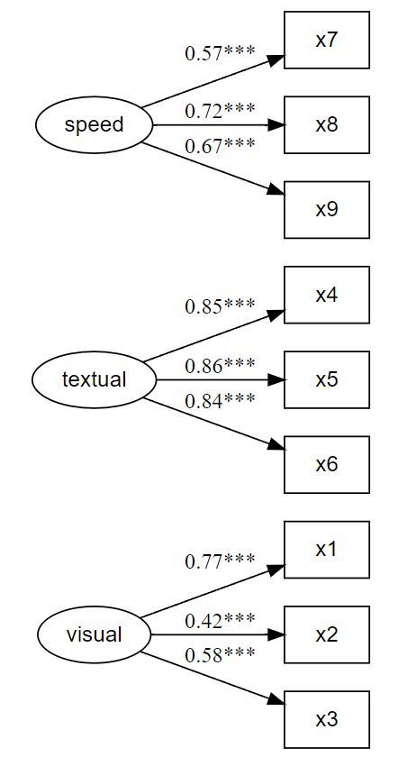
# Get fit indices
nice_fit(fit.cfa)
## Model chisq df chi2.df pvalue cfi tli rmsea rmsea.ci.lower
## 1 Model 1 85.306 24 3.554 0 0.931 0.896 0.092 0.071
## rmsea.ci.upper srmr aic bic
## 1 0.114 0.055 7517.49 7595.339
# We can get it prettier with the `rempsyc::nice_table` integration
nice_fit(fit.cfa, nice_table = TRUE)
Model |
χ2 |
df |
χ2∕df |
p |
CFI |
TLI |
RMSEA [90% CI] |
SRMR |
AIC |
BIC |
|---|---|---|---|---|---|---|---|---|---|---|
Model 1 |
85.31 |
24 |
3.55 |
< .001 |
.93 |
.90 |
.09 [.07, .11] |
.06 |
7,517.49 |
7,595.34 |
Common guidelinesa |
— |
— |
< 2 or 3 |
> .05 |
≥ .95 |
≥ .95 |
< .05 [.00, .08] |
≤ .08 |
Smaller |
Smaller |
aBased on Schreiber (2017), Table 3. | ||||||||||
But let’s say you wanted to develop a short-scale with only x items per dimension. You could decide to remove, for each dimension, the items with the lowest loadings to reach your desired number of items per dimension (but have a look at the Estimation of items reliability section below). You can do so without have to respecify the model, only what items you wish to remove:
# Fit the model fit and plot with `lavaanExtra::cfa_fit_plot`
# to get the factor loadings visually (as PDF)
fit.cfa2 <- cfa_fit_plot(cfa.model, HolzingerSwineford1939,
  remove.items = x[c(2, 6:7)]
)
## lavaan 0.6-20 ended normally after 36 iterations
##
## Estimator ML
## Optimization method NLMINB
## Number of model parameters 15
##
## Number of observations 301
##
## Model Test User Model:
## Standard Scaled
## Test Statistic 13.109 13.560
## Degrees of freedom 6 6
## P-value (Chi-square) 0.041 0.035
## Scaling correction factor 0.967
## Yuan-Bentler correction (Mplus variant)
##
## Model Test Baseline Model:
##
## Test statistic 481.386 460.467
## Degrees of freedom 15 15
## P-value 0.000 0.000
## Scaling correction factor 1.045
##
## User Model versus Baseline Model:
##
## Comparative Fit Index (CFI) 0.985 0.983
## Tucker-Lewis Index (TLI) 0.962 0.958
##
## Robust Comparative Fit Index (CFI) 0.984
## Robust Tucker-Lewis Index (TLI) 0.961
##
## Loglikelihood and Information Criteria:
##
## Loglikelihood user model (H0) -2538.118 -2538.118
## Scaling correction factor 1.076
## for the MLR correction
## Loglikelihood unrestricted model (H1) -2531.563 -2531.563
## Scaling correction factor 1.045
## for the MLR correction
##
## Akaike (AIC) 5106.235 5106.235
## Bayesian (BIC) 5161.842 5161.842
## Sample-size adjusted Bayesian (SABIC) 5114.271 5114.271
##
## Root Mean Square Error of Approximation:
##
## RMSEA 0.063 0.065
## 90 Percent confidence interval - lower 0.012 0.015
## 90 Percent confidence interval - upper 0.109 0.112
## P-value H_0: RMSEA <= 0.050 0.276 0.255
## P-value H_0: RMSEA >= 0.080 0.309 0.337
##
## Robust RMSEA 0.064
## 90 Percent confidence interval - lower 0.016
## 90 Percent confidence interval - upper 0.109
## P-value H_0: Robust RMSEA <= 0.050 0.262
## P-value H_0: Robust RMSEA >= 0.080 0.314
##
## Standardized Root Mean Square Residual:
##
## SRMR 0.036 0.036
##
## Parameter Estimates:
##
## Standard errors Sandwich
## Information bread Observed
## Observed information based on Hessian
##
## Latent Variables:
## Estimate Std.Err z-value P(>|z|) Std.lv Std.all
## visual =~
## x1 1.000 0.954 0.818
## x3 0.637 0.119 5.343 0.000 0.608 0.538
## textual =~
## x4 1.000 1.115 0.959
## x5 0.883 0.140 6.292 0.000 0.985 0.764
## speed =~
## x8 1.000 0.511 0.505
## x9 1.754 0.398 4.405 0.000 0.896 0.889
##
## Covariances:
## Estimate Std.Err z-value P(>|z|) Std.lv Std.all
## visual ~~
## textual 0.472 0.098 4.798 0.000 0.444 0.444
## speed 0.274 0.073 3.732 0.000 0.562 0.562
## textual ~~
## speed 0.144 0.055 2.590 0.010 0.252 0.252
##
## Variances:
## Estimate Std.Err z-value P(>|z|) Std.lv Std.all
## .x1 0.448 0.172 2.606 0.009 0.448 0.330
## .x3 0.905 0.085 10.670 0.000 0.905 0.710
## .x4 0.107 0.190 0.564 0.573 0.107 0.080
## .x5 0.690 0.160 4.311 0.000 0.690 0.416
## .x8 0.761 0.088 8.623 0.000 0.761 0.745
## .x9 0.213 0.165 1.294 0.196 0.213 0.210
## visual 0.910 0.197 4.623 0.000 1.000 1.000
## textual 1.243 0.219 5.678 0.000 1.000 1.000
## speed 0.261 0.080 3.270 0.001 1.000 1.000
##
## R-Square:
## Estimate
## x1 0.670
## x3 0.290
## x4 0.920
## x5 0.584
## x8 0.255
## x9 0.790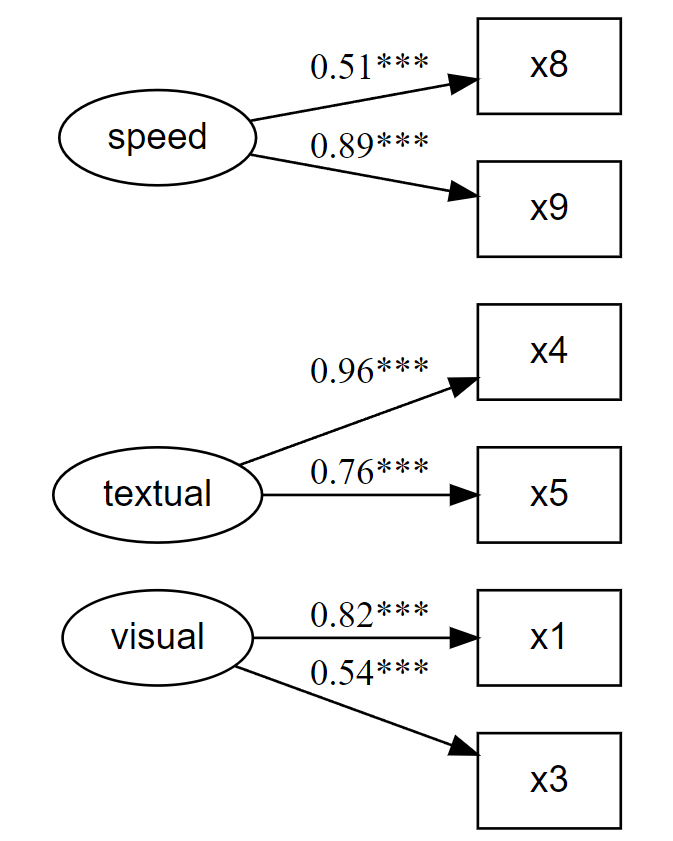
Let’s compare the fit with this short version:
Model |
χ2 |
df |
χ2∕df |
p |
CFI |
TLI |
RMSEA [90% CI] |
SRMR |
AIC |
BIC |
|---|---|---|---|---|---|---|---|---|---|---|
fit.cfa |
85.31 |
24 |
3.55 |
< .001 |
.93 |
.90 |
.09 [.07, .11] |
.06 |
7,517.49 |
7,595.34 |
fit.cfa2 |
13.11 |
6 |
2.19 |
.041 |
.98 |
.96 |
.06 [.01, .11] |
.03 |
5,106.23 |
5,161.84 |
Common guidelinesa |
— |
— |
< 2 or 3 |
> .05 |
≥ .95 |
≥ .95 |
< .05 [.00, .08] |
≤ .08 |
Smaller |
Smaller |
aBased on Schreiber (2017), Table 3. | ||||||||||
If you like this table, you may also wish to save it to Word. Also easy:
# Save fit table to Word!
flextable::save_as_docx(fit_table, path = "fit_table.docx")
Note that it will also render to PDF in an rmarkdown
document with output: pdf_document, but using
latex_engine: xelatex is necessary when including Unicode
symbols in tables like with the nice_fit() function.
Estimation of items reliability
Ideally, rather than just looking at the loadings, we would also
estimate the item reliability of our dimensions for our long vs short
scales to help select which items to drop for our short scale. We can
first look at the alpha when an item is dropped using the
psych::alpha function.
visual <- HolzingerSwineford1939[x[1:3]]
textual <- HolzingerSwineford1939[x[4:6]]
speed <- HolzingerSwineford1939[x[7:9]]

alpha(visual)
##
## Reliability analysis
## Call: alpha(x = visual)
##
## raw_alpha std.alpha G6(smc) average_r S/N ase mean sd median_r
## 0.63 0.63 0.54 0.36 1.7 0.037 4.4 0.88 0.34
##
## 95% confidence boundaries
## lower alpha upper
## Feldt 0.55 0.63 0.69
## Duhachek 0.55 0.63 0.70
##
## Reliability if an item is dropped:
## raw_alpha std.alpha G6(smc) average_r S/N alpha se var.r med.r
## x1 0.51 0.51 0.34 0.34 1.03 0.057 NA 0.34
## x2 0.61 0.61 0.44 0.44 1.58 0.045 NA 0.44
## x3 0.46 0.46 0.30 0.30 0.85 0.062 NA 0.30
##
## Item statistics
## n raw.r std.r r.cor r.drop mean sd
## x1 301 0.77 0.77 0.58 0.45 4.9 1.2
## x2 301 0.73 0.72 0.47 0.37 6.1 1.2
## x3 301 0.78 0.78 0.62 0.48 2.3 1.1
alpha(textual)##
## Reliability analysis
## Call: alpha(x = textual)
##
## raw_alpha std.alpha G6(smc) average_r S/N ase mean sd median_r
## 0.88 0.88 0.84 0.72 7.7 0.011 3.2 1.1 0.72
##
## 95% confidence boundaries
## lower alpha upper
## Feldt 0.86 0.88 0.90
## Duhachek 0.86 0.88 0.91
##
## Reliability if an item is dropped:
## raw_alpha std.alpha G6(smc) average_r S/N alpha se var.r med.r
## x4 0.83 0.84 0.72 0.72 5.1 0.019 NA 0.72
## x5 0.83 0.83 0.70 0.70 4.8 0.020 NA 0.70
## x6 0.84 0.85 0.73 0.73 5.5 0.018 NA 0.73
##
## Item statistics
## n raw.r std.r r.cor r.drop mean sd
## x4 301 0.90 0.90 0.82 0.78 3.1 1.2
## x5 301 0.92 0.91 0.84 0.79 4.3 1.3
## x6 301 0.89 0.90 0.81 0.77 2.2 1.1
alpha(speed)##
## Reliability analysis
## Call: alpha(x = speed)
##
## raw_alpha std.alpha G6(smc) average_r S/N ase mean sd median_r
## 0.69 0.69 0.6 0.43 2.2 0.031 5 0.81 0.45
##
## 95% confidence boundaries
## lower alpha upper
## Feldt 0.62 0.69 0.74
## Duhachek 0.63 0.69 0.75
##
## Reliability if an item is dropped:
## raw_alpha std.alpha G6(smc) average_r S/N alpha se var.r med.r
## x7 0.62 0.62 0.45 0.45 1.6 0.044 NA 0.45
## x8 0.51 0.51 0.34 0.34 1.0 0.057 NA 0.34
## x9 0.65 0.65 0.49 0.49 1.9 0.040 NA 0.49
##
## Item statistics
## n raw.r std.r r.cor r.drop mean sd
## x7 301 0.79 0.78 0.59 0.49 4.2 1.1
## x8 301 0.82 0.82 0.69 0.57 5.5 1.0
## x9 301 0.75 0.76 0.55 0.46 5.4 1.0Looking at the “Reliability if an item is dropped” section, we can see that our decision to drop items 2, 6, and 7, is consistent with these new results except for item 7. Indeed, according to this reliability estimation, it would be better to drop item 9 instead.
SEM example
Here is a structural equation model example. We start with a path analysis first.
Saturated model
One might decide to look at the saturated lavaan model
first.
# Calculate scale averages
data <- HolzingerSwineford1939
data$visual <- rowMeans(data[x[1:3]])
data$textual <- rowMeans(data[x[4:6]])
data$speed <- rowMeans(data[x[7:9]])

# Define our variables
M <- "visual"
IV <- c("ageyr", "grade")
DV <- c("speed", "textual")

# Define our lavaan lists
mediation <- list(speed = M, textual = M, visual = IV)
regression <- list(speed = IV, textual = IV)
covariance <- list(speed = "textual", ageyr = "grade")

# Write the model, and check it
model.saturated <- write_lavaan(
  mediation = mediation,
  regression = regression,
  covariance = covariance
)
cat(model.saturated)
## ##################################################
## # [-----------Mediations (named paths)-----------]
##
## speed ~ visual
## textual ~ visual
## visual ~ ageyr + grade
##
## ##################################################
## # [---------Regressions (Direct effects)---------]
##
## speed ~ ageyr + grade
## textual ~ ageyr + grade
##
## ##################################################
## # [------------------Covariances-----------------]
##
## speed ~~ textual
## ageyr ~~ gradeThis looks good so far, but we might also want to check our indirect
effects (mediations). For this, we have to obtain the path names by
setting label = TRUE. This will allow us to define our
indirect effects and feed them back to write_lavaan.
# We can run the model again.
# However, we set `label = TRUE` to get the path names
model.saturated <- write_lavaan(
  mediation = mediation,
  regression = regression,
  covariance = covariance,
  label = TRUE
)
cat(model.saturated)
## ##################################################
## # [-----------Mediations (named paths)-----------]
##
## speed ~ visual_speed*visual
## textual ~ visual_textual*visual
## visual ~ ageyr_visual*ageyr + grade_visual*grade
##
## ##################################################
## # [---------Regressions (Direct effects)---------]
##
## speed ~ ageyr + grade
## textual ~ ageyr + grade
##
## ##################################################
## # [------------------Covariances-----------------]
##
## speed ~~ textual
## ageyr ~~ gradeHere, if we check the mediation section of the model, we see that it
has been “augmented” with the path names. Those are
visual_speed, visual_textual,
ageyr_visual, and grade_visual. The logic for
the determination of the path names is predictable: it is always the
predictor variable, on the left, followed by the predicted variable, on
the right. So if we were to test all possible indirect effects, we would
define our indirect object as such:
# Define indirect object
indirect <- list(
  ageyr_visual_speed = c("ageyr_visual", "visual_speed"),
  ageyr_visual_textual = c("ageyr_visual", "visual_textual"),
  grade_visual_speed = c("grade_visual", "visual_speed"),
  grade_visual_textual = c("grade_visual", "visual_textual")
)

# Write the model, and check it
model.saturated <- write_lavaan(
  mediation = mediation,
  regression = regression,
  covariance = covariance,
  indirect = indirect,
  label = TRUE
)
cat(model.saturated)
## ##################################################
## # [-----------Mediations (named paths)-----------]
##
## speed ~ visual_speed*visual
## textual ~ visual_textual*visual
## visual ~ ageyr_visual*ageyr + grade_visual*grade
##
## ##################################################
## # [---------Regressions (Direct effects)---------]
##
## speed ~ ageyr + grade
## textual ~ ageyr + grade
##
## ##################################################
## # [------------------Covariances-----------------]
##
## speed ~~ textual
## ageyr ~~ grade
##
## ##################################################
## # [--------Mediations (indirect effects)---------]
##
## ageyr_visual_speed := ageyr_visual * visual_speed
## ageyr_visual_textual := ageyr_visual * visual_textual
## grade_visual_speed := grade_visual * visual_speed
## grade_visual_textual := grade_visual * visual_textualIf preferred (e.g., when dealing with long variable names), one can choose to use letters for the predictor variables. Note however that this tends to be somewhat more confusing and ambiguous.
# Write the model, and check it
model.saturated <- write_lavaan(
  mediation = mediation,
  regression = regression,
  covariance = covariance,
  label = TRUE,
  use.letters = TRUE
)
cat(model.saturated)
## ##################################################
## # [-----------Mediations (named paths)-----------]
##
## speed ~ a_speed*visual
## textual ~ a_textual*visual
## visual ~ a_visual*ageyr + b_visual*grade
##
## ##################################################
## # [---------Regressions (Direct effects)---------]
##
## speed ~ ageyr + grade
## textual ~ ageyr + grade
##
## ##################################################
## # [------------------Covariances-----------------]
##
## speed ~~ textual
## ageyr ~~ gradeIn this case, the path names are a_speed,
a_textual, a_visual, and
b_visual. So we would define our indirect
object as such:
# Define indirect object
indirect <- list(
  ageyr_visual_speed = c("a_visual", "a_speed"),
  ageyr_visual_textual = c("a_visual", "a_textual"),
  grade_visual_speed = c("b_visual", "a_speed"),
  grade_visual_textual = c("b_visual", "a_textual")
)

# Write the model, and check it
model.saturated <- write_lavaan(
  mediation = mediation,
  regression = regression,
  covariance = covariance,
  indirect = indirect,
  label = TRUE,
  use.letters = TRUE
)
cat(model.saturated)
## ##################################################
## # [-----------Mediations (named paths)-----------]
##
## speed ~ a_speed*visual
## textual ~ a_textual*visual
## visual ~ a_visual*ageyr + b_visual*grade
##
## ##################################################
## # [---------Regressions (Direct effects)---------]
##
## speed ~ ageyr + grade
## textual ~ ageyr + grade
##
## ##################################################
## # [------------------Covariances-----------------]
##
## speed ~~ textual
## ageyr ~~ grade
##
## ##################################################
## # [--------Mediations (indirect effects)---------]
##
## ageyr_visual_speed := a_visual * a_speed
## ageyr_visual_textual := a_visual * a_textual
## grade_visual_speed := b_visual * a_speed
## grade_visual_textual := b_visual * a_textualThere is also an experimental feature that attempts to produce the
indirect effects automatically. This feature requires specifying your
independent, dependent, and mediator variables as “IV”, “M”, and “DV”,
respectively, in the indirect object. In our case, we have
already defined those earlier, so we can just feed the proper
objects.
# Define indirect object
indirect <- list(IV = IV, M = M, DV = DV)

# Write the model, and check it
model.saturated <- write_lavaan(
  mediation = mediation,
  regression = regression,
  covariance = covariance,
  indirect = indirect,
  label = TRUE
)
cat(model.saturated)
## ##################################################
## # [-----------Mediations (named paths)-----------]
##
## speed ~ visual_speed*visual
## textual ~ visual_textual*visual
## visual ~ ageyr_visual*ageyr + grade_visual*grade
##
## ##################################################
## # [---------Regressions (Direct effects)---------]
##
## speed ~ ageyr + grade
## textual ~ ageyr + grade
##
## ##################################################
## # [------------------Covariances-----------------]
##
## speed ~~ textual
## ageyr ~~ grade
##
## ##################################################
## # [--------Mediations (indirect effects)---------]
##
## ageyr_visual_speed := ageyr_visual * visual_speed
## ageyr_visual_textual := ageyr_visual * visual_textual
## grade_visual_speed := grade_visual * visual_speed
## grade_visual_textual := grade_visual * visual_textualWe are now satisfied with our model, so we can finally fit it!
# Fit the model with `lavaan`
fit.saturated <- sem(model.saturated, data = data)

# Get regression parameters only
# And make it pretty with the `rempsyc::nice_table` integration
lavaan_reg(fit.saturated, nice_table = TRUE, highlight = TRUE)
Outcome |
Predictor |
SE |
Z |
p |
b |
95% CI (b) |
b* |
95% CI (b*) |
|---|---|---|---|---|---|---|---|---|
speed |
visual |
0.05 |
3.91 |
< .001*** |
0.20 |
[0.10, 0.29] |
0.21 |
[0.11, 0.31] |
textual |
visual |
0.06 |
4.53 |
< .001*** |
0.29 |
[0.16, 0.41] |
0.24 |
[0.14, 0.34] |
visual |
ageyr |
0.05 |
-2.47 |
.014* |
-0.13 |
[-0.24, -0.03] |
-0.16 |
[-0.29, -0.03] |
visual |
grade |
0.11 |
4.31 |
< .001*** |
0.49 |
[0.27, 0.72] |
0.28 |
[0.16, 0.40] |
speed |
ageyr |
0.05 |
0.57 |
.568 |
0.03 |
[-0.07, 0.12] |
0.04 |
[-0.09, 0.16] |
speed |
grade |
0.10 |
4.90 |
< .001*** |
0.50 |
[0.30, 0.70] |
0.31 |
[0.19, 0.43] |
textual |
ageyr |
0.06 |
-6.72 |
< .001*** |
-0.41 |
[-0.52, -0.29] |
-0.40 |
[-0.51, -0.29] |
textual |
grade |
0.13 |
5.87 |
< .001*** |
0.76 |
[0.51, 1.01] |
0.36 |
[0.24, 0.47] |
So speed as predicted by ageyr isn’t
significant. We could remove that path from the model it if we are
trying to make a more parsimonious model. Let’s make the non-saturated
path analysis model next.
Path analysis model
Because we use lavaanExtra, we don’t have to redefine
the entire model: simply what we want to update. In this case, the
regressions and the indirect effects.
regression <- list(speed = "grade", textual = IV)

# We can run the model again, setting `label = TRUE` to get the path names
model.path <- write_lavaan(
  mediation = mediation,
  regression = regression,
  covariance = covariance,
  label = TRUE
)
cat(model.path)
## ##################################################
## # [-----------Mediations (named paths)-----------]
##
## speed ~ visual_speed*visual
## textual ~ visual_textual*visual
## visual ~ ageyr_visual*ageyr + grade_visual*grade
##
## ##################################################
## # [---------Regressions (Direct effects)---------]
##
## speed ~ grade
## textual ~ ageyr + grade
##
## ##################################################
## # [------------------Covariances-----------------]
##
## speed ~~ textual
## ageyr ~~ grade
# We check that we have removed "ageyr" correctly from "speed" in the
# regression section. OK.
# Define just our indirect effects of interest
indirect <- list(
age_visual_speed = c("ageyr_visual", "visual_speed"),
grade_visual_textual = c("grade_visual", "visual_textual")
)
# We run the model again, with the indirect effects
model.path <- write_lavaan(
mediation = mediation,
regression = regression,
covariance = covariance,
indirect = indirect,
label = TRUE
)
cat(model.path)## ##################################################
## # [-----------Mediations (named paths)-----------]
##
## speed ~ visual_speed*visual
## textual ~ visual_textual*visual
## visual ~ ageyr_visual*ageyr + grade_visual*grade
##
## ##################################################
## # [---------Regressions (Direct effects)---------]
##
## speed ~ grade
## textual ~ ageyr + grade
##
## ##################################################
## # [------------------Covariances-----------------]
##
## speed ~~ textual
## ageyr ~~ grade
##
## ##################################################
## # [--------Mediations (indirect effects)---------]
##
## age_visual_speed := ageyr_visual * visual_speed
## grade_visual_textual := grade_visual * visual_textual
# Fit the model with `lavaan`
fit.path <- sem(model.path, data = data)
# Get regression parameters only
lavaan_reg(fit.path)## Outcome Predictor SE Z p b CI_lower
## 1 speed visual 0.04967204 3.861565 1.126628e-04 0.1918118 0.09445643
## 2 textual visual 0.06336429 4.518796 6.219227e-06 0.2863303 0.16213859
## 3 visual ageyr 0.05439452 -2.469906 1.351486e-02 -0.1343493 -0.24096064
## 4 visual grade 0.11439571 4.306175 1.661018e-05 0.4926079 0.26839646
## 5 speed grade 0.08716854 6.111181 9.889656e-10 0.5327027 0.36185552
## 6 textual ageyr 0.05979047 -6.851140 7.326362e-12 -0.4096329 -0.52682005
## 7 textual grade 0.12908567 5.925622 3.111173e-09 0.7649129 0.51190965
## CI_upper B CI_lower_B CI_upper_B
## 1 0.28916724 0.2064640 0.1035674 0.30936052
## 2 0.41052205 0.2351233 0.1353706 0.33487606
## 3 -0.02773804 -0.1610061 -0.2876179 -0.03439429
## 4 0.71681940 0.2807072 0.1566382 0.40477626
## 5 0.70354992 0.3267428 0.2271881 0.42629750
## 6 -0.29244571 -0.4031160 -0.5133146 -0.29291740
## 7 1.01791619 0.3579255 0.2434470 0.47240398
# We can get it prettier with the `rempsyc::nice_table` integration
lavaan_reg(fit.path, nice_table = TRUE, highlight = TRUE)Outcome |
Predictor |
SE |
Z |
p |
b |
95% CI (b) |
b* |
95% CI (b*) |
|---|---|---|---|---|---|---|---|---|
speed |
visual |
0.05 |
3.86 |
< .001*** |
0.19 |
[0.09, 0.29] |
0.21 |
[0.10, 0.31] |
textual |
visual |
0.06 |
4.52 |
< .001*** |
0.29 |
[0.16, 0.41] |
0.24 |
[0.14, 0.33] |
visual |
ageyr |
0.05 |
-2.47 |
.014* |
-0.13 |
[-0.24, -0.03] |
-0.16 |
[-0.29, -0.03] |
visual |
grade |
0.11 |
4.31 |
< .001*** |
0.49 |
[0.27, 0.72] |
0.28 |
[0.16, 0.40] |
speed |
grade |
0.09 |
6.11 |
< .001*** |
0.53 |
[0.36, 0.70] |
0.33 |
[0.23, 0.43] |
textual |
ageyr |
0.06 |
-6.85 |
< .001*** |
-0.41 |
[-0.53, -0.29] |
-0.40 |
[-0.51, -0.29] |
textual |
grade |
0.13 |
5.93 |
< .001*** |
0.76 |
[0.51, 1.02] |
0.36 |
[0.24, 0.47] |
# We only kept significant regressions. Good (for this demo).
# Get correlations
lavaan_cor(fit.path)## Variable 1 Variable 2 SE Z p sigma CI_lower
## 8 speed textual 0.04017743 2.254287 2.417812e-02 0.09057145 0.01182514
## 9 ageyr grade 0.03401916 7.885426 3.108624e-15 0.26825556 0.20157923
## CI_upper r CI_lower_r CI_upper_r
## 8 0.1693178 0.1312679 0.02005915 0.2424766
## 9 0.3349319 0.5113296 0.42775726 0.5949020
# We can get it prettier with the `rempsyc::nice_table` integration
lavaan_cor(fit.path, nice_table = TRUE)Variable 1 |
Variable 2 |
SE |
Z |
p |
σ |
95% CI (σ) |
r |
95% CI (r) |
|---|---|---|---|---|---|---|---|---|
speed |
textual |
0.04 |
2.25 |
.024* |
0.09 |
[0.01, 0.17] |
.13 |
[0.02, 0.24] |
ageyr |
grade |
0.03 |
7.89 |
< .001*** |
0.27 |
[0.20, 0.33] |
.51 |
[0.43, 0.59] |
# Get nice fit indices with the `rempsyc::nice_table` integration
nice_fit(lst(fit.cfa, fit.saturated, fit.path), nice_table = TRUE)Model |
χ2 |
df |
χ2∕df |
p |
CFI |
TLI |
RMSEA [90% CI] |
SRMR |
AIC |
BIC |
|---|---|---|---|---|---|---|---|---|---|---|
fit.cfa |
85.31 |
24 |
3.55 |
< .001 |
.93 |
.90 |
.09 [.07, .11] |
.06 |
7,517.49 |
7,595.34 |
fit.saturated |
0.00 |
0 |
Inf |
1.0 |
1.0 |
.00 [.00, .00] |
.00 |
3,483.46 |
3,539.02 |
|
fit.path |
0.33 |
1 |
0.33 |
.568 |
1.0 |
1.3 |
.00 [.00, .13] |
-.00 |
3,481.79 |
3,533.64 |
Common guidelinesa |
— |
— |
< 2 or 3 |
> .05 |
≥ .95 |
≥ .95 |
< .05 [.00, .08] |
≤ .08 |
Smaller |
Smaller |
aBased on Schreiber (2017), Table 3. | ||||||||||
# Let's get the indirect effects only
lavaan_defined(fit.path, lhs_name = "Indirect Effect")## Indirect Effect Paths SE Z
## 15 age → visual → speed ageyr_visual*visual_speed 0.01238517 -2.080697
## 16 grade → visual → textual grade_visual*visual_textual 0.04524584 3.117383
## p b CI_lower CI_upper B CI_lower_B
## 15 0.037461652 -0.02576979 -0.05004429 -0.001495299 -0.03324196 -0.06438407
## 16 0.001824646 0.14104859 0.05236837 0.229728799 0.06600083 0.02535014
## CI_upper_B
## 15 -0.002099853
## 16 0.106651508
# We can get it prettier with the `rempsyc::nice_table` integration
lavaan_defined(fit.path, lhs_name = "Indirect Effect", nice_table = TRUE)Indirect Effect |
Paths |
SE |
Z |
p |
b |
95% CI (b) |
b* |
95% CI (b*) |
|---|---|---|---|---|---|---|---|---|
age → visual → speed |
ageyr_visual*visual_speed |
0.01 |
-2.08 |
.037* |
-0.03 |
[-0.05, -0.00] |
-0.03 |
[-0.06, -0.00] |
grade → visual → textual |
grade_visual*visual_textual |
0.05 |
3.12 |
.002** |
0.14 |
[0.05, 0.23] |
0.07 |
[0.03, 0.11] |
# Get modification indices only
modindices(fit.path, sort = TRUE, maximum.number = 5)## lhs op rhs mi epc sepc.lv sepc.all sepc.nox
## 29 visual ~ textual 0.326 1.622 1.622 1.975 1.975
## 35 grade ~ textual 0.326 -0.228 -0.228 -0.488 -0.488
## 34 grade ~ speed 0.326 -0.038 -0.038 -0.062 -0.062
## 19 speed ~~ grade 0.326 -0.021 -0.021 -0.056 -0.056
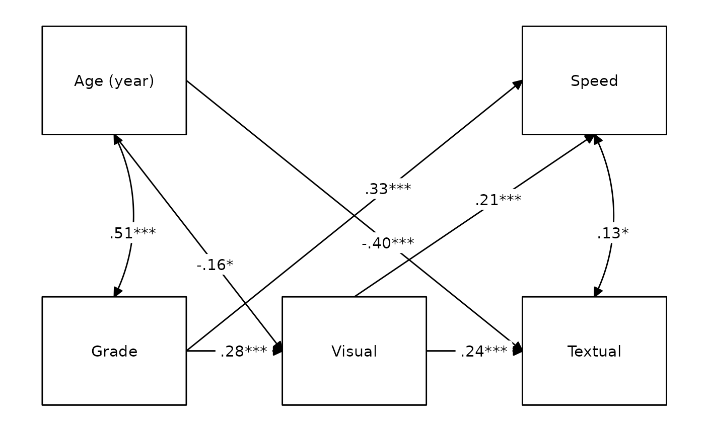
## 25 speed ~ textual 0.326 -0.067 -0.067 -0.087 -0.087For reference, this is our model, visually speaking
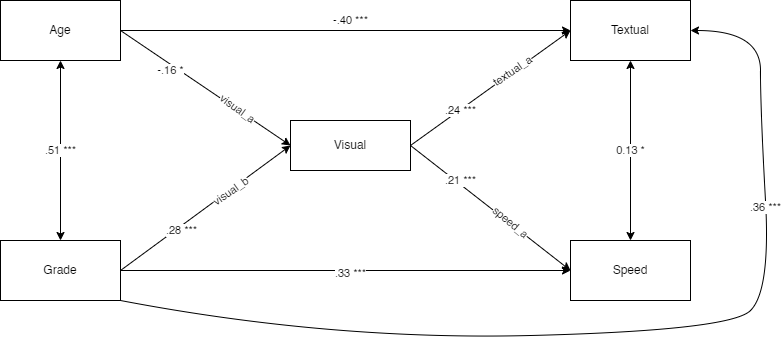
We could also attempt to draw it with
lavaanExtra::nice_tidySEM, a convenience wrapper around the
amazing tidySEM package.
labels <- list(
ageyr = "Age (year)",
grade = "Grade",
visual = "Visual",
speed = "Speed",
textual = "Textual"
)
layout <- list(IV = IV, M = M, DV = DV)
nice_tidySEM(fit.path,
layout = layout, label = labels,
hide_nonsig_edges = TRUE, label_location = .60
)
Latent model
Finally, perhaps we change our mind and decide to run a full SEM instead, with latent variables. Fear not: we don’t have to redo everything again. We can simply define our latent variables and proceed. In this example, we have already defined our latent variable for our CFA earlier, so we don’t even need to write that again!
model.latent <- write_lavaan(
mediation = mediation,
regression = regression,
covariance = covariance,
indirect = indirect,
latent = latent,
label = TRUE
)
cat(model.latent)## ##################################################
## # [-----Latent variables (measurement model)-----]
##
## visual =~ x1 + x2 + x3
## textual =~ x4 + x5 + x6
## speed =~ x7 + x8 + x9
##
## ##################################################
## # [-----------Mediations (named paths)-----------]
##
## speed ~ visual_speed*visual
## textual ~ visual_textual*visual
## visual ~ ageyr_visual*ageyr + grade_visual*grade
##
## ##################################################
## # [---------Regressions (Direct effects)---------]
##
## speed ~ grade
## textual ~ ageyr + grade
##
## ##################################################
## # [------------------Covariances-----------------]
##
## speed ~~ textual
## ageyr ~~ grade
##
## ##################################################
## # [--------Mediations (indirect effects)---------]
##
## age_visual_speed := ageyr_visual * visual_speed
## grade_visual_textual := grade_visual * visual_textual
# Run model
fit.latent <- sem(model.latent, data = HolzingerSwineford1939)

# Get nice fit indices with the `rempsyc::nice_table` integration
nice_fit(lst(fit.cfa, fit.saturated, fit.path, fit.latent), nice_table = TRUE)
Model |
χ2 |
df |
χ2∕df |
p |
CFI |
TLI |
RMSEA [90% CI] |
SRMR |
AIC |
BIC |
|---|---|---|---|---|---|---|---|---|---|---|
fit.cfa |
85.31 |
24 |
3.55 |
< .001 |
.93 |
.90 |
.09 [.07, .11] |
.06 |
7,517.49 |
7,595.34 |
fit.saturated |
0.00 |
0 |
Inf |
1.0 |
1.0 |
.00 [.00, .00] |
.00 |
3,483.46 |
3,539.02 |
|
fit.path |
0.33 |
1 |
0.33 |
.568 |
1.0 |
1.3 |
.00 [.00, .13] |
-.00 |
3,481.79 |
3,533.64 |
fit.latent |
118.92 |
37 |
3.21 |
< .001 |
.92 |
.89 |
.09 [.07, .10] |
.05 |
8,638.79 |
8,746.20 |
Common guidelinesa |
— |
— |
< 2 or 3 |
> .05 |
≥ .95 |
≥ .95 |
< .05 [.00, .08] |
≤ .08 |
Smaller |
Smaller |
aBased on Schreiber (2017), Table 3. | ||||||||||