Make a quick tidySEM plot — nice_tidySEM • lavaanExtra

Make a quick and decent-looking tidySEM plot.

Usage

nice_tidySEM(
  fit,
  layout = NULL,
  hide_nonsig_edges = FALSE,
  hide_var = TRUE,
  hide_cov = FALSE,
  hide_mean = TRUE,
  est_std = TRUE,
  label,
  label_location = NULL,
  reduce_items = NULL,
  plot = TRUE,
  ...
)

Arguments

fit: SEM or CFA model fit to plot.
layout: A matrix (or data.frame) that describes the structure; see tidySEM::get_layout. If a named list is provided, with names "IV" (independent variables), "M" (mediator), and "DV" (dependent variables), nice_tidySEM attempts to write the layout matrix automatically.
hide_nonsig_edges: Logical, hides non-significant edges. Defaults to FALSE.
hide_var: Logical, hides variances. Defaults to TRUE.
hide_cov: Logical, hides co-variances. Defaults to FALSE.
hide_mean: Logical, hides means/node labels. Defaults to TRUE.
est_std: Logical, whether to use the standardized coefficients. Defaults to TRUE.
label: Labels to be used on the plot. As elsewhere in lavaanExtra, it is provided as a named list with format (colname = "label").
label_location: Location of label along the path, as a percentage (defaults to middle, 0.5).
reduce_items: A numeric vector of length 1 (x) or 2 (x & y) defining how much space to trim from the nodes (boxes) of the items defining the latent variables. Can be provided either as reduce_items = 0.4 (will only affect horizontal space, x), or reduce_items = c(x = 0.4, y = 0.2) (will affect both horizontal x and vertical y).
plot: Logical, whether to plot the result (default). If FALSE, returns the tidy_sem object, which can be further edited as needed.
...: Arguments to be passed to tidySEM::prepare_graph.

Value

A tidySEM plot, of class ggplot, representing the specified lavaan model.

Illustrations

Examples

# Calculate scale averages
library(lavaan)
data <- HolzingerSwineford1939
data$visual <- rowMeans(data[paste0("x", 1:3)])
data$textual <- rowMeans(data[paste0("x", 4:6)])
data$speed <- rowMeans(data[paste0("x", 7:9)])

# Define our variables
IV <- c("sex", "ageyr", "agemo", "school")
M <- c("visual", "grade")
DV <- c("speed", "textual")

# Define our lavaan lists
mediation <- list(speed = M, textual = M, visual = IV, grade = IV)

# Define indirect object
structure <- list(IV = IV, M = M, DV = DV)

# Write the model, and check it
model <- write_lavaan(mediation, indirect = structure, label = TRUE)
cat(model)
#> ##################################################
#> # [-----------Mediations (named paths)-----------]
#> 
#> speed ~ visual_speed*visual + grade_speed*grade
#> textual ~ visual_textual*visual + grade_textual*grade
#> visual ~ sex_visual*sex + ageyr_visual*ageyr + agemo_visual*agemo + school_visual*school
#> grade ~ sex_grade*sex + ageyr_grade*ageyr + agemo_grade*agemo + school_grade*school
#> 
#> ##################################################
#> # [--------Mediations (indirect effects)---------]
#> 
#> sex_visual_speed := sex_visual * visual_speed
#> sex_visual_textual := sex_visual * visual_textual
#> ageyr_visual_speed := ageyr_visual * visual_speed
#> ageyr_visual_textual := ageyr_visual * visual_textual
#> agemo_visual_speed := agemo_visual * visual_speed
#> agemo_visual_textual := agemo_visual * visual_textual
#> school_visual_speed := school_visual * visual_speed
#> school_visual_textual := school_visual * visual_textual
#> sex_grade_speed := sex_grade * grade_speed
#> sex_grade_textual := sex_grade * grade_textual
#> ageyr_grade_speed := ageyr_grade * grade_speed
#> ageyr_grade_textual := ageyr_grade * grade_textual
#> agemo_grade_speed := agemo_grade * grade_speed
#> agemo_grade_textual := agemo_grade * grade_textual
#> school_grade_speed := school_grade * grade_speed
#> school_grade_textual := school_grade * grade_textual
#> 

# Fit model
fit <- sem(model, data)

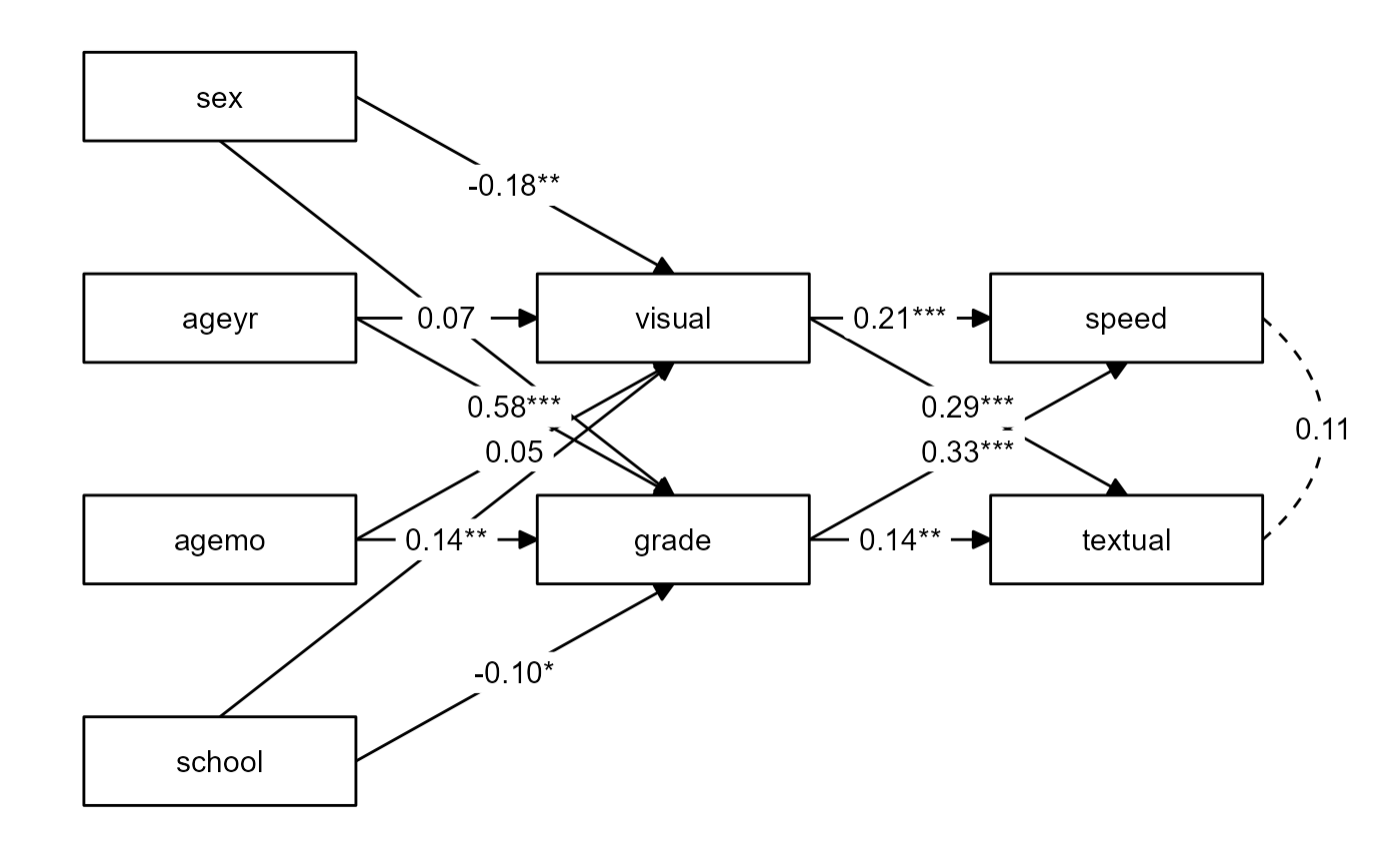
# Plot model
# \donttest{
nice_tidySEM(fit, layout = structure)

# }
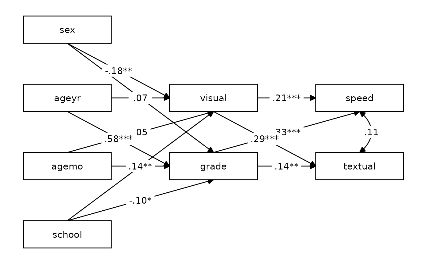